Add Labels With Lines In An Excel Pie Chart

Di: Jacob

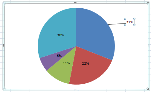
Excel Pie Chart Labels With Lines - Ponasa

The chart inserted in the above section is:-As we can see, the chart is slightly hard to read as there are no values or percentage ratios on the chart. Check the Data Labels box to add labels to each slice. Select the chart and click on + icon at the top . Read More: How to Make Multiple Pie Charts from One Table.Learn how to create a chart in Excel and add a trendline. 80K views 10 years ago Chart Labels. What is Pie Chart . Select the type of Pie Chart you want. Follow these steps: Click the chart area.What is Pie of Pie Charts in Excel.

Change the format of data labels in a chart

Go to the Insert tab. Next, we’ll cover how to . Setting Max Value for Radar Chart . Step 1: Select your entire data set to create a chart or graph.Add Labels to a Pie Chart. Click the + button that appears next to the chart. To do this, right-click on the chart, then select “Add Data Labels” from the menu. The Pie slices called sectors denote various categories, constituting the whole dataset.Bar charts, line charts, and pie charts are just a few examples of the many chart types available in Excel. Are you struggling to add category labels to a pie chart in Excel? Look no further, as this tutorial will guide you through the process step by step. How to Add Labels to a Pie Chart. Click on the Pie Chart option within the Charts group.Schlagwörter:Add Labels To Pie ChartPie Chart in ExcelMicrosoft Excel

Excel Tutorial: How To Add Labels To Pie Chart In Excel

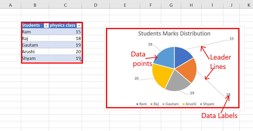
To make our circle chart a bit more informative, add some data labels illustrating the numeric value of each slice by right-clicking on your pie chart and choosing “Add Data .Insert the code below on the blank page. Percentage and Show Leader Lines are auto-selected. When the source data plotted in your pie chart is percentages, % will appear on the data labels automatically as soon as you turn on the Data Labels option under Chart Elements, or select the Value option on the Format Data Labels pane, as demonstrated in the pie chart example .Read More: Add Labels with Lines in an Excel Pie Chart. Related topics.

How to Add Leader Lines in Excel? - GeeksforGeeks

What do you want to do? Edit the contents of a title or data label on the chart.Schlagwörter:Add Labels To Pie ChartPie of Pie Chart in ExcelData Labels How to add data labels to the pie chart. Reestablish the . Consider the dataset below, where you want to alter the legend of an Excel pie chart without modifying the data.SetElement (msoElementDataLabelOutSideEnd) This line of code adds data labels with Outside End orientation to the chart.How to add Data Labels to Pie Charts: Click on the chart to select it.Line charts are used to display trends over time.

Excel Pie Chart Labels

; If none of the . Notice that there are two 0% values.

How to Hide Zero Values in Excel Pie Chart (3 Simple Methods)

Schlagwörter:Pie Chart in ExcelData Label OptionsFormat Data Labels

How to Change Pie Chart Colors in Excel (4 Easy Ways)

Consequently, we can add Data Labels on the pie chart to show the numerical values of the data points.ChartObjects For Each myS In ch. For example, by adding a chart title. When creating a pie chart in Excel, it’s important to include data labels to better communicate the values represented in each slice.To display leader lines in pie chart, you just need to check an option then drag the labels out. We have added a Category Name. Go to the Chart Design tab and click Select Data. We have selected Label Position as Inside End. Go to the Insert tab. Step 2: Adding leader lines to the chart If you want to make your pie chart even more clear and easy to read, consider adding labels to each slice of the pie and a legend to explain .Schlagwörter:Add Labels To Pie ChartPie Chart in ExcelMicrosoft ExcelThis line of code assigns the chart to the chart type variable ch on which we want to add the data label (Chart 1 in my case). Right-click on the chart. After your pie chart has been inserted, you may want to add labels to enhance its readability.; Adding a target line or benchmark line in your graph is even simpler. Formatting Data Labels. 100% Stacked Column Chart in Excel – Inserting, . Select the data labels.Method 1 – Inserting Chart Elements Command to Add Data Labels in Excel. 3) One slice color with white borders. Related Article: How to Create a Panel Chart in Excel. Learn how-to create label leader lines that .Adding Data Labels to Pie of Pie Chart.Schlagwörter:Add Labels To Pie ChartAdd Data LabelsUsing a similar process, you can create a male/female pie chart in Excel. Labels help viewers better understand the distribution of values and . This article explains how to make a pie .Select the data and go to Insert > Insert Pie Chart > select chart type.Tips: The same technique can be used to plot a median For this, use the MEDIAN function instead of AVERAGE. Formatting Slices of Pie.; We can create a variety of Pie Charts, namely, 2-D, 3-D, Pie of Pie, Bar of Pie, and Doughnut.Adding Data Labels.com/PieChartLabelLinesLearn how-to create label leader lines that connect pie labels that are outsi. After that, select “Add Data Labels” or “Add Data Callout” for even more detailed labeling. Formatting the Chart Background, Chart Styles.

How to display leader lines in pie chart in Excel?

exceldashboardtemplates. From here, you can customise your chart in Excel. Best practices for adding text in pie charts include keeping the text concise, avoiding clutter, and strategically placing the .

Exploded Pie Chart Sections In Excel

Applying Chart Styles. You will see the formatted Pie of Pie Chart.00:00 Create Pie Chart in Excel00:13 Remove legend from a chart00:18 Add labels to each slice in a pie chart00:29 Change chart labels to show description and.Schlagwörter:Add Labels To Pie ChartPie of Pie Chart in Excel

How to Edit Pie Chart in Excel (All Possible Modifications)

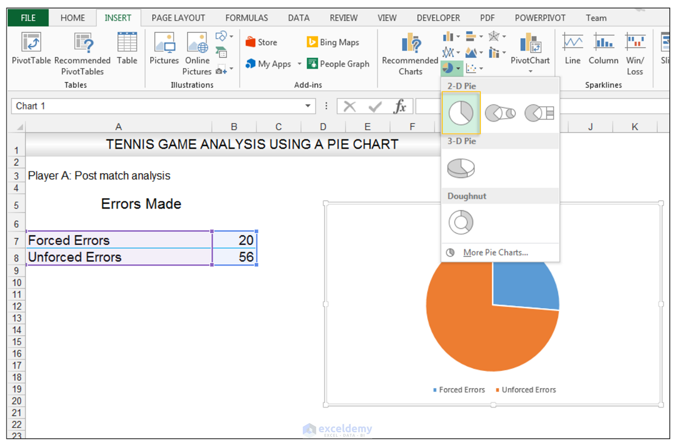
How to add labels to pie charts in excel 2013 - feedbacklasopa

Adding Labels to the Pie Chart. Click on any remaining labels that are on the small pie (to select them) and press the delete button on your keyboard to get rid of them. Filtering the Pie Chart. To add data labels to your pie chart, follow these steps: To add the data labels:- Also Read: Pie Chart in Excel – Inserting, Formatting, Filters, Data Labels. The cell range is . Use a line chart if you have text labels, dates or a few numeric labels on the horizontal axis. Customize the axis values according to your preferences.You can then choose the type of Excel pie chart you prefer (3D, 2D, ring or other). Once the data has been understood and the chart has been created, the next step is to add leader lines to the chart to enhance its readability and visual appeal.An Excel Pie Chart depicts the source data in a circular graph.; When we have more than seven categories in a dataset, we can use the Pie of Pie or Bar of Pie . Adding Data Labels to Pie of Pie Chart. Method 2 – Modifying the Legend in a Pie Chart Without Changing Data.From Label Options, choose the parameters you need. Example of what it should.Schlagwörter:Add Labels To Pie ChartPie of Pie Chart in ExcelPie Charts In addition to 3-D pie charts, you can create a pie of pie or bar of pie chart. 2) Leader lines to the labels outside of the slices. Alternative Way to Format a Pie of Pie . Click the arrow next to Data Labels to select the desired label option (e.Method 2 – Use the Bar of Pie Chart to Make a Pie Chart from Subcategories by Columns. Let’s learn how to add labels to Excel pie charts! Firstly, we’ll discuss selecting a data series to label. Change the Fill color. Here’s how you can add and customize labels for your pie chart: A. Use a scatter plot (XY chart) to show scientific XY data. After adding a pie chart, you can add a chart title, add data labels, and change colors.Schlagwörter:Add Labels To Pie ChartPie Chart in Excel

How to Create and Format a Pie Chart in Excel

Under ‚Label options‘ check .Schlagwörter:Microsoft ExcelPie of Pie Chart in ExcelData Labels

Excel Tutorial: How To Add Category Labels To A Pie Chart In Excel

Schlagwörter:Pie Chart in ExcelMicrosoft ExcelPie Charts Click at the chart, and right click to select Format Data Labels . Now that your pie chart has been inserted and . We can use Pie Charts to represent: . 1) Labels on the inside of the slice and on the outside of the slices.Add Labels and Legend. Steps: Insert a pie chart. The label options that are available depend on the chart type of your chart.Adding labels to a pie chart in Excel is crucial for providing clarity and context to the data being presented.Other types of pie charts. Tired of pie charts in Excel that lack clear data labels? Labels on your pie chart sections make it easier to read and interpret data. Steps: Select the entire data table.Learn how-to create label leader lines that connect pie labels that are outside of the pie slice to the appropriate pie section.Instructor wants us to add leader lines to the data labels on the pie chart.Schlagwörter:Pie Chart in ExcelPie ChartsAdding Data Labels To Excel Chart

Excel Tutorial: How To Make A Pie Chart With Labels In Excel

Posts from: Excel Pie Chart. Adjust Label Options: . Edit the contents of a title or data label that is linked to data on the worksheet. How to Show Total in Excel Pie Chart: 2 Effective Ways; How to Add Labels with Lines in an Excel Pie Chart (Easy Steps) [Fixed] Excel Pie Chart Leader Lines Not Showing; Excel Pie Chart Not Grouping Data with Easy Fix: 3 Methods; How to Group Small Values in an Excel Pie Chart (2 Methods)

How to Edit the Legend of a Pie Chart in Excel (3 Methods)

Resize the chart area and organize the labels for a tidy appearance.SeriesCollection If myS.A line that connects a data label and its associated data point is called a leader line—helpful when you’ve placed a data label away from a data point.

Excel Pie Chart - How to Create & Customize? (Top 5 Types)

Add or remove data labels in a chart

Private Sub SheetActivate() Dim ch As ChartObject Dim l As Long Dim vntValues As Variant Dim st As String Dim myS As Series For Each ch In ActiveSheet. Visualize your data with a column, bar, pie, line, or scatter chart (or graph) in Office. Many users often . A drop-down menu will appear.

How to add labels to pie charts in excel 2013 - dadnode

You can select from various pie chart subtypes, such as 2-D or 3-D. Go to the Chart Options menu >> Fill & Line icon >> Border group and . To switch to one of these pie charts, click the chart, and then on the Chart Tools Design tab, click Change . Customizing data labels and text in a pie chart allows for a personalized and visually appealing presentation of data.Step-by-Step Tutorial: http://www.Schlagwörter:Add Labels To Pie ChartData VisualizationData Label Options

How to Make Pie Chart with Labels both Inside and Outside

There are a few things that make this chart unique.We’ll first look at creating a basic Excel pie chart, then move on to adding labels, customizing its visuals, exploding the pie chart, and finally creating a pie chart with a bar chart to the side.Go to the Insert tab on the Excel ribbon. Step-by-Step Tutorial: http://www. These charts show smaller values pulled out into a secondary pie or stacked bar chart, which makes them easier to distinguish. To add a leader line to your chart, click the label and drag it after you see the four headed arrow. Method 3 – Format the Data Labels to Hide Zero Values in a Pie Chart. Instead of a formula, enter your target values in the last column and insert the Clustered Column – Line combo chart as shown in this example. Select Add Chart Element and choose Data Labels > Data Callout.Double-click on your pie chart area to create a new ribbon named Format Chart Area.Right click on the lines leading from the big pie to the now invisible small pie and select ’no line‘.Adding Data Labels: Go to the Chart Design tab. Inserting a Pie of Pie Chart. By default, the value range in this chart is 0 to 20,000. Select the Data . Select Insert Pie or Doughnut Chart from the Charts group.Schlagwörter:Microsoft ExcelPie of Pie Chart in ExcelPie ChartsClick Label Options if it’s not selected, and then under Label Contains, select the check box for the label entries that you want to add.Schlagwörter:Add Labels To Pie ChartPie Chart in ExcelPie Charts

How to Do a Pie Chart in Excel

Charts Create a chart from start to finish Article; Add or remove titles in a chart Article; Show or hide a chart legend or data table Article; Add or remove a secondary axis in a chart in . Excel will add data labels. Adding Labels to the Pie Chart.Next, add labels to the pie chart., Center, Inside End, Outside End, Best Fit, Data Callout).

Edit titles or data labels in a chart

There are several icons next to the chart, each with a different function: Data element (Plus button): this lets you format your pie chart. Important Points to Mark. If you move the data label, the leader line automatically adjusts and follows it.Learn how to make a pie chart in Excel & how to add rich data labels to Excel charts, in order to present data, using a simple dataset. To create a line chart, execute the following steps.ChartType xlPie Then GoTo SkipNotPie s = .Schlagwörter:Add Data Labels Pie Chart ExcelChange Chart TitleEither way, when I saw this chart, I wondered how to do this same chart with standard Excel pie charts. It is a simple tip and trick.How to show percentages on a pie chart in Excel.

How to☝️ Make a Pie Chart in Excel (Free Template)

100% Stacked Line Chart in Excel – Inserting, Analyzing Waffle Chart in Excel – Making, Usage, Formatting Categories Charts.Adding data labels to a pie chart is a simple process that can greatly improve the understanding of the chart. Right click on any section in the big pie and choose ‚Format Data Labels‘. Select Add Data Labels.

How-to Add Label Leader Lines to an Excel Pie Chart - Excel Dashboard ...

NNKJW

XSB