Conditional Format To Apply If Different Formula Is Used
Di: Jacob
To guide you, in this article, we will discuss 6 different ways that you can use to apply conditional formatting to the .Conditional Formatting is a versatile and flexible tool embedded in Excel that enables us to modify and format cells based on various conditions. Learn to create and add conditional formatting rules, including using formulas, with this workbook full of examples. It can help you highlight the most important information in your spreadsheets and spot variances of cell values with a quick glance. Let’s start with an example: Criteria 1: Cell Value Is Greater Than Particular Value.IF Formula – Set Cell Color w/ Conditional Formatting – Excel & Google Sheets. Experiment on your own and use other formulas you are familiar with.
Conditional Formatting
The BIG thing revealed in that Q&A was the use of the ‚$‘ sign in the custom formula.
How to Apply Conditional Formatting in Excel If Another
) and mixed references.In this article, you will get the easiest ways to do conditional formatting for multiple conditions in Excel.This Tutorial Covers: Using Conditional Formatting in Excel (Examples) 1.Count > 1 Then IsFormula = CVErr(xlErrNA)Else IsFormula = Ref. Download the workbook. Now that we have the logic nailed down, it’s time to set it up as a Conditional Formatting rule. The first table has the sales record for different items of a companyIf you are looking for a different approach, I have also posted an article on How to find duplicates in two excel sheets.> Enter the above formula in Edit Rule Description window> Choose the Format Fill to preview and press OK Please note that you have to fix the column by making it absolute using $ sign with it, and keep the row number free or relative to change. This tutorial will demonstrate how to highlight cells depending on the answer returned by an IF .See more on superuserFeedbackVielen Dank!Geben Sie weitere Informationen anSchlagwörter:Apply Conditional FormattingMicrosoft ExcelMicrosoft Office
Conditional formatting with formulas
We have the two data tables, which we’ll format. Highlight Cells with Value Greater/Less than a Number. i want to make a conditional formatting rule for color scales, so it evaluates the ranking for each item across all columns so i can rank sales for each item by month.
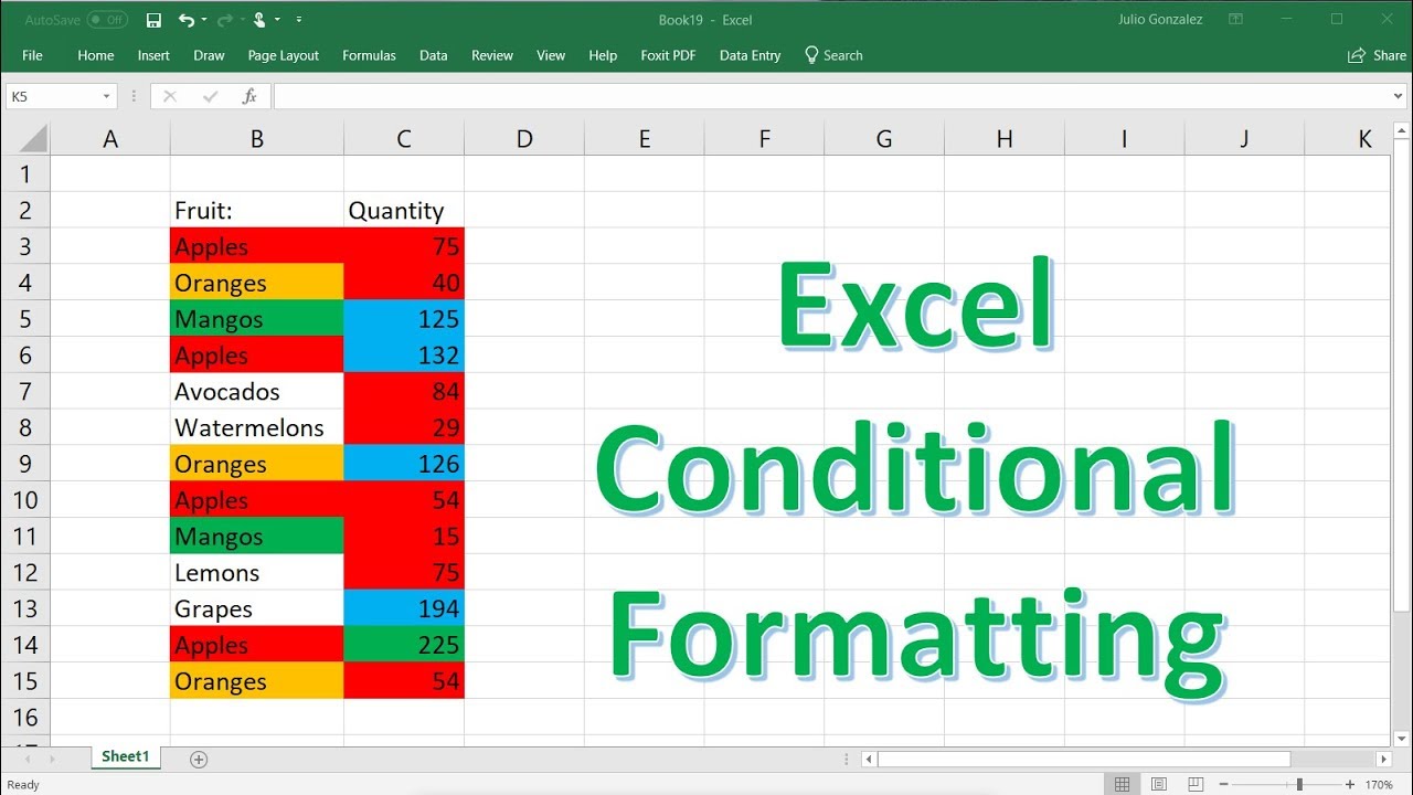
i could only get excel to evaluate by rows (so all item numbers were being ranked . I use the color Green for the > and the color Red for the <. In this article, I am going to show you some examples where you can apply Conditional . Conditional Formatting is a very versatile tool. With Conditional Formatting, we will show you how to highlight rows in different colors based on multiple conditions by adding 2 rules using the Conditional Formatting Rules Manager.Use a formula to determine which cells to format. Find cells that have conditional formatting. It has pre-defined conditions but you can also use formulas for more complex tasks. In the examples above, we used very simple formulas for conditional formatting.
How to Use Conditional Formatting to Highlight Text in Excel
Every time the rules are saved it will always display A1 on Sheet A in red.- Click OK to apply the changes and close the dialog boxes.Other Options with Icon Sets.
Compare data in a cell outside the conditionally formatted range of cells.Using a Formula for Conditional Formatting to Highlight a Row.Conditional Formatting will apply the formula to the whole dataset.Google Sheets: selecting cell values based on another cell . In the example shown, the formula used to apply conditional . Copy and paste conditional formatting. Highlight Cells Rules . Insert the following formula in the Format values where this formula is true cell: =B5= B5 is the first cell of the order date. There, you can choose pre-set options or create formulas for your needs.Use conditional formatting to highlight information.The formatting is applied to column C.
Conditional Formatting to Highlight Rows in Excel
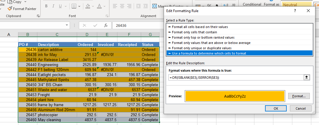
You apply conditional formatting with what is called conditional formatting rules.Based on different criteria, we’ll apply formatting rules to this dataset. Many users, especially beginners, find it intricate and obscure.So, the icon for the highest value will move to the lowest value. There are many of conditions based on which we can format cells in many ways. In the sample data, I want to identify all L compatible adapters.This tutorial demonstrates how to apply conditional formatting based on a formula in Excel and Google Sheets.Weitere Ergebnisse anzeigen Click here to open a view-only copy >> Feel free to make a copy: File > Make a copy. Select Use a formula to determine which cells to format, and enter the formula: .
Conditional Formatting Not Equal
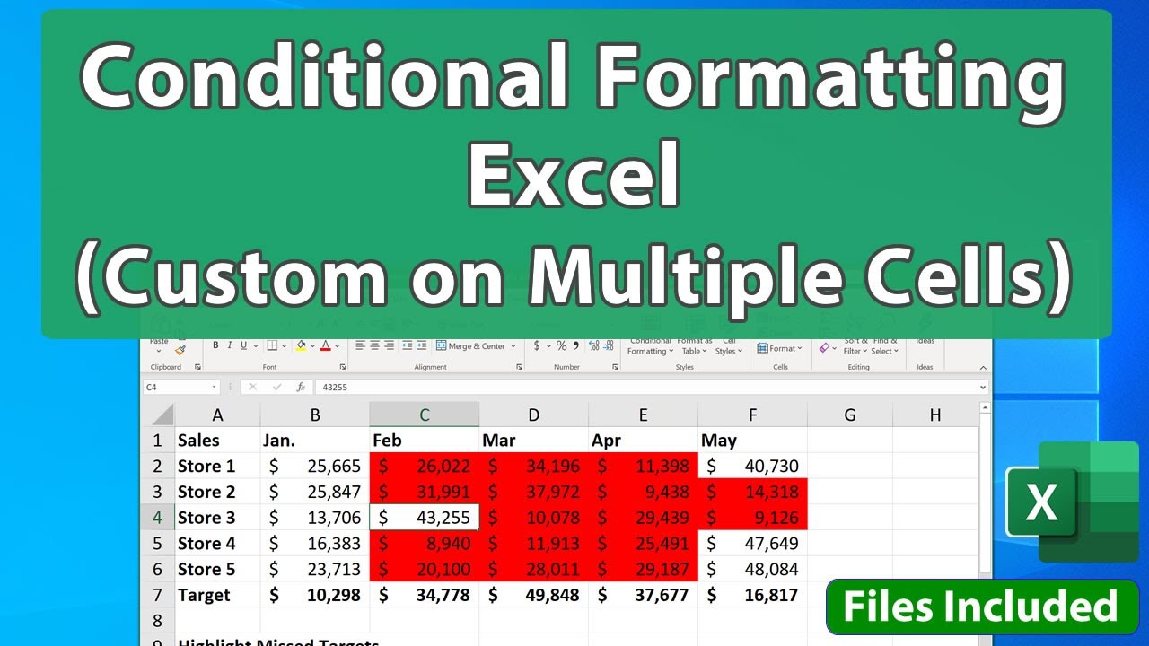
That can also be done using the formula technique in Conditional Formatting. Conditional Formatting in Excel comes with plenty of preset . How to find duplicates in Excel.You won’t be able to use conditional formatting to do this. Click on the Format option from the lower-right corner of the dialog box.To apply conditional formatting based on a value in another column, you can create a rule based on a simple formula. In this example, I am going to format the cells in the Product column if the corresponding cell in the In stock column is greater than 300. Select the cell range F6:F13.
How to Apply Conditional Formatting to the Selected Cells
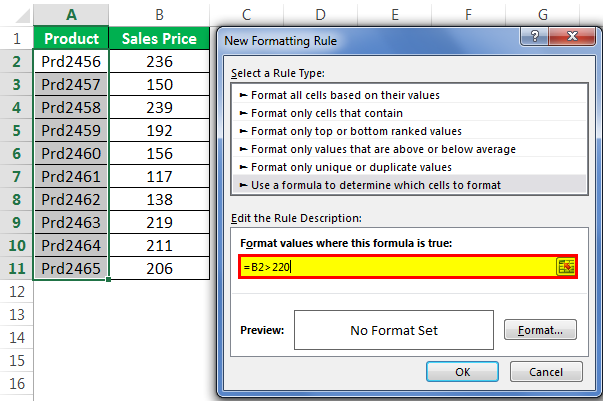
It’s really easy to insert one of those. Let’s start with an example: Criteria 1: Cell .In the dialog box, New Formatting Rule, choose the option Use a formula to determine which cells to format as a Rule Type. And some of the useful examples that you can use in your daily work. Training: To control more precisely what cells will be formatted, you can use formulas to apply . The steps to apply CF with formulas are quite simple: Select the range to apply Conditional Formatting. You can pick an entire row, column or some cells. Quickly Identify Duplicates. Go to the Home tab, click on Conditional . Type the following data table into your workbook. Go to the “Home” tab and click on “Conditional Formatting”.To highlight cells whose values are not equal to a specific value, you can create a Conditional Formatting custom formula using the following steps: Select the range you want to apply formatting to. What I’m saying is sometimes another question may not necessarily resolve one’s question, .Select the cells you want to apply conditional formatting rules to. Method 3 – Using the COUNTIF Function in Conditional Formatting for More Than Two Columns. You can highlight cells based on specific rules, such as greater than, lesser than, or within a certain range. Select all the cells where the text you want to highlight can be. The first criterion we will add is to search column D .Using other sheets in conditional formatting is not supported.Conditional Formatting With Multiple Conditions.
To manage these rules, you should understand the order in which these rules are evaluated, what happens when two or more rules conflict, how copying and pasting can affect rule evaluation, how to change the order in which . Excel already provides a means of highlighting formulas that are inconsistent with others in the same region : File . Show Icon Only: When you tick mark this option, this will hide the values from the range and show only the icons that you have. Start in cell A1. Select Use a formula to determine which cells to format, and enter the formula: =IF(B4>5,TRUE,FALSE) Click the Format button and select your desired formatting. In the middle of the Home tab, click ‘Conditional .Conditional Formatting (on the Home tab) > New Rule> Use a formula to determine. Move the cursor over the Fill .So today in this post, I’d like to share with you simple steps to apply conditional formatting using a formula. In addition, – Use Paste (Ctrl+V) or Paste Special and choose Formats or Formulas and Formatting to copy the conditional formatting along with the value. Manage conditional formatting rule precedence. To highlight cells according to multiple conditions being met, you can use the IF and AND Functions within a conditional .
Conditional Formatting If Cell Contains Specific Text
Steps to Apply Conditional Formatting with Formulas.
Excel conditional formatting formulas based on another cell
Reverse Icon Order: While applying icon formatting, you can change the order of the icons in reverse. Is the function wrong? Or is it not possible to have a Conditional Format even search across sheets? This checks that your data looks as intended.Excel conditional formatting is a really powerful feature when it comes to applying different formats to data that meets certain conditions.So the formula to apply conditional formatting to entire columns is: =A$1=Client This rule checks for client in row 1 and if it finds client, the formatting is applied to the whole of that column: Conditional Formatting Template. To update the formula, follow these steps: Select the cells with your data (cells A6 to B20). Manage conditional formatting rules. Shade an entire row where several criteria must . In the example shown, conditional formatting is applied to the range B5:B12 using 3 formulas: =B5>=90% // green =B5>=80% // yellow =B5
How To Sort Or Filter By Conditional Format Results In Excel
To highlight the differences between two columns of data with conditional formatting you can use a simple formula that uses the not equal to operator (e.Advanced types of conditional formatting in Excel. If you can’t access the template, it might . Select the range you want to apply formatting to. Shade alternate rows in a range.
Conditionally format a range based on a different range
Adding conditional formatting in Excel allows you to apply different formatting options to a cell, or range of cells, that meet specific conditions that you set. You can find the Conditional Formatting in the Home tab, under the .Select the range you want to apply formatting to. As a workaround: Clone the data from SheetB in SheetA using =SheetB!A1, use e.Each rule will have its own color and criterion.
How to use Icon Sets in Excel (Conditional Formatting)
Remember: We always use the formula created in the UPPER-LEFT corner of the test area.I’ve been playing around with the Conditional Formatting Rules Manager and have a rule set to the formula ISTEXT(A&ROW())=TRUE and if I statically set cells in the Applies to .Highlight Rows in Different Colors Based on Multiple Conditions. Preview your changes before applying them. In the Ribbon, select Home > Conditional Formatting > New Rule.; Icon Style: You can change the .To highlight a percentage value in a cell using different colors, where each color represents a particular level, you can use multiple conditional formatting rules, with each rule targeting a different threshold.
IF Formula
Excel Conditional Formatting Based on Another Cell
To highlight cells with certain text defined in another cell, you can use a formula in Conditional Formatting. Click OK, then OK again to return to the Conditional . Highlight Cells Rules.Use conditional formatting. Here’s one more example if you want to take it to the next level.To control more precisely what cells will be formatted, you can use formulas to apply conditional formatting.Here’s an overview of using Conditional Formatting for multiple conditions.When you use conditional formatting, you set up rules that Excel uses to determine when to apply the conditional formatting. columns Y+ [Hide columns Y+] .
:max_bytes(150000):strip_icc()/ApplyingMultipleRulesinExcel-5bf0518846e0fb0058244268.jpg)

Conditional Formatting Based on Formula
So, I select all cells in column B (from cell B2 and down). If it uses absolute references, consider changing them . Now that we have seen the basic uses of conditional formatting in Excel, let’s explore more advanced options that will let you customize the rules according to your specific needs.How do I include formatting (colour) when I link cells .

How to Use Conditional Formatting with IF Statement
how about if i have months listed in a table, columns A – L ,and item numbers in the rows with sales for each month.
Applying Conditional Formatting for Multiple Conditions in Excel
Check the conditional formatting formula in the original cell. I had to experiment with combinations to have the condition apply to a whole row, but I haven’t seen any discussion else on that topic.HasFormulaEnd If.Quick Start
Conditional formatting based on another column
Setting such conditions .@kando You may be right, but I’m not sure.Under the custom formula I use: =A1>(SheetB!A1), but it doesn’t seem to work.
- Dasauge® Stellenmarkt | Stellenangebot: Senior Art Director (m/w/x) (Berlin)
- Einwegkunststofffondverordnung
- Personalize O Design De Um Modelo De Carta
- Raphael Mechoulam, Pionier Der Cannabis-Forschung
- Machtausübung Und Kontrolle , Machtausübung und Kontrolle positiv einsetzen
- Wie Bei Der Bank Ausweisen? , Bonn-Ausweis: bequem und bürger*innenfreundlich
- Seit Einer Dekade | mag seit einer Dekade haaren
- Möbelleder Und Polsterleder [Lederpedia
- Diagnose Stecker | Wo ist der OBD Stecker im Audi A4
- Obe Tv Bedeutung , Was ist der Unterschied zwischen OBE, MBE, CBE und Knighthood?
- 10秒解决Steam社区出现Ssl错误代码无法进入的教程 | steam社区打不开、显示错误代码的解决方法
- Becher · Dick · Hrsg. Völker, Reiche Und Namen Im Frühen Mittelalter
- Nationalmannschaft: Joachim Löw Und Die Türkei-Connection